Next: Step 3 - Projection of the QTL, Previous: Step 1 - Creating the XML Database, Up: Tutorial
For clarity, and to avoid to put all the output files into the current directory, create a directory called meta-map into which files related to the consensus map construction will be stored.
Before creating the consensus map using the program ConsMap, it is important to check if the input maps are consistent between them. Consistency means here that: i) it must exist a path of common markers which connects the same chromosomes in the different input maps, ii) the marker order must be globally conserved between input maps which share more than 1 common marker.
To get a first diagnostic of the nature of the marker connection bewteen input maps run the command InfoMap as follows:
$java org.metaqtl.main.InfoMap -m xml -o meta-map/infomap -t 2 |
-t to 2, in order to discard the markers which are not common between maps.
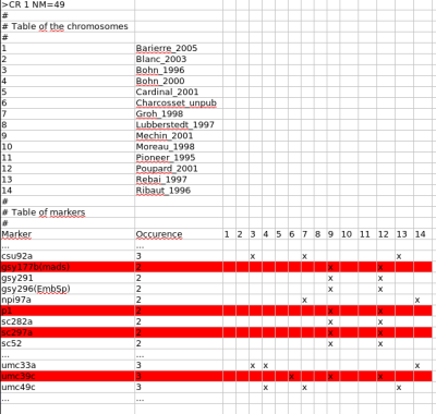
Then go into the directory meta-map. There are now two files:
     >CR 1 Connected=true
     #
     # Table of the chromosomes
     #
     1       Barierre_2005   3       71.4333333333333
     2       Blanc_2003      11      20.563636363636366
     3       Bohn_1996       10      16.9
     4       Bohn_2000       12      25.166666666666597
     5       Cardinal_2001   12      18.908333333333342
     6       Charcosset_unpub        11      23.181818181818194
     7       Groh_1998       13      17.415384615384614
     8       Lubberstedt_1997        6       44.666666666666764
     9       Mechin_2001     20      12.900000000000006
     10      Moreau_1998     8       24.74999999999999
     11      Pioneer_1995    9       30.45555555555556
     12      Poupard_2001    26      10.600000000000025
     13      Rebai_1997      18      15.833333333333364
     14      Ribaut_1996     11      24.18181818181821
The fact that the attribute Connected is equal to true means that it exists a path between common markers which connects all the chromosome together (in other words, a consensus chromosome one can be built using ConsMap). The follows the average marker interval distance in the 14 input mapping experiments - not 18 because for 4 of them there is no information about chromosome 1.
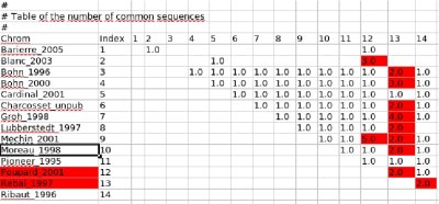
Now, have a look to the table called "Table of the number of common marker sequences" below:
MMapView.
Let's start with the pairwise comparison between the genetic maps of experiments Poupard_2001 and Mechin_2001. First create the directory images into meta-map and run the following command line:
     $java org.metaqtl.main.MMapView -r xml/Poupard_2001.xml -m xml/Mechin_2001.xml \
                                     -c 1 --mrkt 2 -o meta-map/images/PoupardVSMechin
|
WITH_COMMON_MARKER to true.
WITH_COMMON_MARKER=true
Other parameters can be aslo modified to obtain a better display of the chromosomes. For example:
CHROM_DISTANCE_SCALE=3.0 #�default is 5
COMMON_STROKE_WIDTH=1.0 #�default is 5 (the stroke used to show the common sequences)
LAYER_VSPACE=50.0 #�default is 50 (this increases the space between the chromosomes)
Now move the plot parameter file to meta-map/images/comparison.par (this because we will use the same parameter file for all the comparisons to do) and run the command:
     $java org.metaqtl.main.MMapView -r xml/Poupard_2001.xml -m xml/Mechin_2001.xml \
                                     -c 1 --mrkt 2 -o meta-map/images/PoupardVSMechin \
     				-p meta-map/images/comparison.par
|
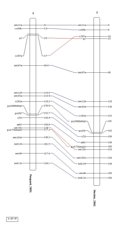
Indeed, there are 3 common sequences in the same order (the blue ones) and two common marker sequences in reverse order (the red ones). We can see that these inversions involve very close markers in both chromosome maps. Besides, if we have a look to the file infomap_mrk.txt we can see that:
only the marker umc39c is observed in another mapping experiment, Charcosset_unpub. So removing a marker per inversion will not degrade the consensus map construction for the chromosome 1.
Then, we create the file mrkrm.txt in the folder meta-map in order to record the two markers to remove
     Mechin_2001	1	p1
     Mechin_2001	1	gsy177b(mads)
     Poupard_2001	1	p1
     Poupard_2001	1	gsy177b(mads)
If we repeat this operation for the other pairwise comparison showing a number of commom marker sequences greater than 1, we can establish a full list of dubious markers to remove (note that in some cases you can update the name of the marker instead of removing it using the option --mrkup in MetaDB):
     Mechin_2001     1       p1
     Mechin_2001     1       gsy177b(mads)
     Poupard_2001    1       p1
     Poupard_2001    1       gsy177b(mads)
     Blanc_2003      1       umc1278
     Poupard_2001    1       umc1278
     Rebai_1997      1       umc11a
     Rebai_1997      1       umc58
     Rebai_1997      1       umc49c
     Ribaut_1996     1       npi97a
     Groh_1998       1       npi97a
Then, we have to run back the command MetaDB with the option --mrkrm to remove these markers from the XML database:
     $java org.metaqtl.main.MetaDB -e data/experiments.csv -m data/genetic-map \
                                   -q data/qtl-map -t data/trait_ontology.csv \
     			      -d data/marker_dictionary.csv -o xml \
     			      --mrkm meta-map/mrkrm.txt
|
InfoMap to see that now there are no longer marker inversions between the chromosome 1 of the different input maps. Of course the operations described in this section must be repeated for all the chromosomes.
When all the marker inversions have been resolved, we can build the consensus map using the command ConsMap.
$java org.metaqtl.main.ConsMap -m xml -o meta-map/consensus |
Then, if we want to display the consensus map in tabulated text format, we can use the command Xml2A as follows:
     $java org.metaqtl.main.Xml2A -x meta-map/consensus_map.xml -t map -f tab \
                                  -o meta-map/consensus_map.txt
|
     map	group	locus	type	position	meta.occurence
     	1	ph1056	M	0	1
     	1	bnlg1124	M	4.71	1
     	1	bnl5.62a	M	6.7	6
     	1	umc164	M	9.98	2
     	1	umc94a	M	11.7	4
     	1	umc1177	M	12.51	1
     	...	...	...	...	...
     	1	umc86a	M	248.82	1
     	1	phi064	M	250.13	1
     	1	phi22756	M	253.6	1
     	1	bnl6.32	M	254.1	9
     	1	umc1797	M	268.5	1
The first column map is empty since by default the consensus map has no name. To add a name to the consensus map you must edit by hand the file consensus_map.xml and to put the suited name of the consensus map into double quoted after the attribute name in the tag genome:
<genome-map name="my_consensus_map">
The last column meta.occurence gives the number of times the marker have been seen into the input mapping experiments on the same chromosome (it should be the same than in the file infomap_mrk.txt previously generated).
Let's plot the histogram of these values.
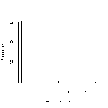
We can see that we have an excess of singleton markers, i.e. of markers which have observed only on a single mapping experiments. So the consensus map must be considered with care. In order to see how this excess of singleton markers can affect the construction of the consensus map, it could be interesting to compare the consensus map with a reference map.
For example, we downloaded from the MaizeGDB web site the reference map called Genetic 2005. This raw text file of this reference map is in the directory data/ref-map and it is called genetic_2005.txt. So, before making the comparison with our consensus map, we have to convert this file into a XML representation. To do so, use the command A2Xml as follows:
     $java org.metaqtl.main.A2Xml -i data/ref-map/genetic_2005.txt -t map -f tab
                                  -o ref-map/genetic_2005.xml
|
To compare our consensus map with the reference map we then use the command MMapView as follows:
     $java org.metaqtl.main.MMapView -m meta-map/consensus_map.xml
                                     -r ref-map/genetic_2005.xml \
                                     -c 1 --mrkt 2 -o meta-map/images/RefVsCons \
     				-p meta-map/images/comparison.par
|
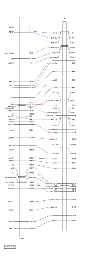
We can see that there are 8 inversions and that some of these inversions are not common sequences (in gray). Now, let's have a look to the occurence of the 11 markers involved in these inversions (into the file consensus_map.txt):
     ...	...	...	...	...
     1	bnl5.62a	M	6.7	6
     ...	...	...	...	...
     1	obf1	M	101.9	1
     1	umc167a	M	102.99	1
     ...	...	...	...	...
     1	csu574b(eif2B)	M	106.04	1
     ...	...	...	...	...
     1	rs2	M	113.45	1
     ...	...	...	...	...
     1	php20644	M	126.38	1
     ...	...	...	...	...
     1	umc58	M	133.3	5
     ...	...	...	...	...
     1	adh1	M	190.34	3
     1	kn1	M	191.32	1
     ...	...	...	...	...
     1	umc107a(croc)	M	196.68	3
     1	csu137b(ap)	M	197.93	1
     ...	...	...	...	...
Now, let's have a look to the way these markers are distributed among the input mapping experiments using the file infomap_mrk.txt (note that if you have kept the option -t set to 2 as in the previous example of the use of InfoMap you need to run again the command by discarding this option in order to get the information for the singleton markers).
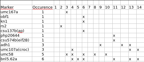
Then, let's remove the 7 singleton markers (add the following list to the file mrkrm.txt previously edited):
     Bohn_1996       1       umc167a
     Blanc_2003      1       rs2
     Charcosset_unpub        1       obf1
     Charcosset_unpub        1       kn1
     Charcosset_unpub        1       csu137b(ap)
     Pioneer_1995    1       php20644
     Pioneer_1995    1       csu574b(eif2B)
Finally, recreate the XML database and rebuild the consensus map
     $java org.metaqtl.main.MetaDB -e data/experiments.csv -m data/genetic-map \
                                   -q data/qtl-map -t data/trait_ontology.csv \
     			      -d data/marker_dictionary.csv -o xml \
     			      --mrkm meta-map/mrkrm.txt
     $java org.metaqtl.main.ConsMap -m xml -o meta-map/consensus
|
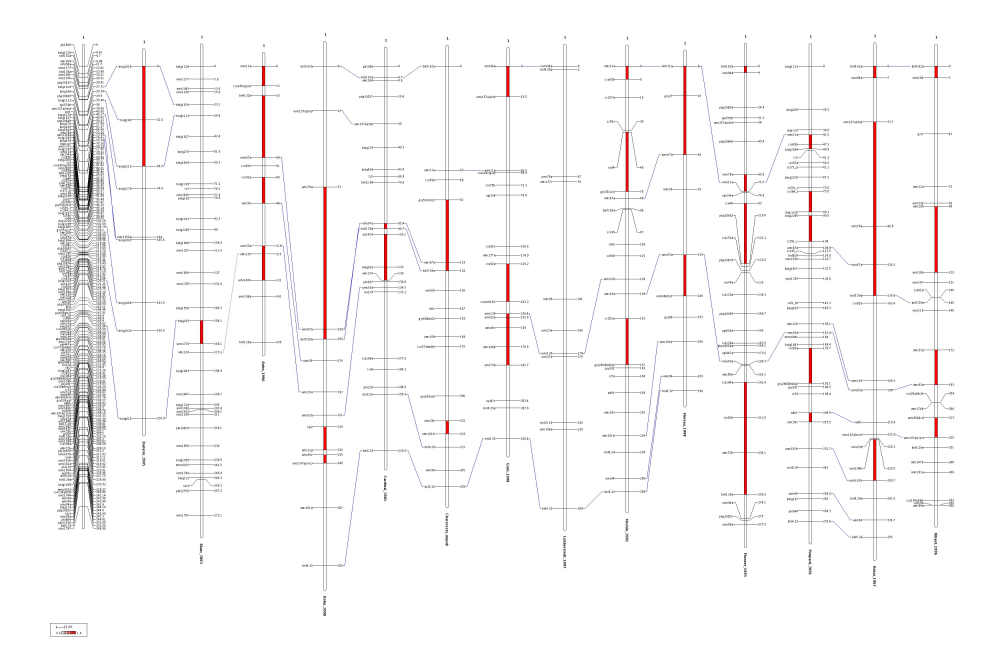
MMapView by setting the options --htest and --hth. The last option --hth allows the user to define the level of the test. For example, if we want to get the marker intervals which standarized residuals are significatively outside the expected distribution at a level of 5\%, we will use the following command:
     $java org.metaqtl.main.MMapView -r meta-map/consensus_map.xml -m xml -c 1 \
                                     -o meta-map/images/ConsensusVSAll \
     				-p meta-map/images/consensus.par \
     				--hth 9.5E-2 --htest
|
--hth must be equal to one minus the level of the test.
Normaly, you will obtain something like that: