6.4 Step 3 - Projection of the QTL

Once the consensus map have been established, we can project all the observed QTL from the initial mapping experiments onto this consensus map. This is a compulsory step to carry out the meta-analysis.

To do so, use the program QTLProj as follows:

$java org.metaqtl.main.QTLProj -m meta-map/consensus_map.xml \ -q xml -o meta-qtl/consensus --verbose [ WARNING ] : Unable to project QTL Rebai_1997_SD_14 on chromosome 2 [ WARNING ] : Unable to project QTL Rebai_1997_SD_27 on chromosome 2 [ WARNING ] : Unable to project QTL Rebai_1997_SD_21 on chromosome 2 [ WARNING ] : Unable to project QTL Rebai_1997_SD_7 on chromosome 2

Note that setting the option --verbose displays the warnings. In this case, it seems that there is a problem with the mapping experiment Rebai_1997 for the chromosome 2. Since here we focus on chromosome 1, we will ignore these warnings for the rest of the tutorial.

This command generates two files into the directory meta-qtl:

• consensus_map.xml: the consensus map plus the projected QTL.
• consensus_qtl.xml: the consensus map with only the projected QTL.

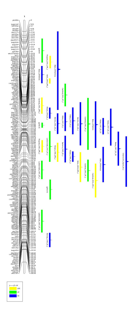
Now, if we want to see how the QTL have been projected and are distributed along the chromosome 1, we can use the command MapView as follows:

java org.metaqtl.main.MapView -m meta-qtl/consensus_map.xml -c 1 \ -o meta-qtl/images/consensus \ -p meta-qtl/images/consensus.par -q

This should give the following picture:

Now, if we want to see the properties of the QTL projection for each QTL we can export the file consensus_qtl.xml into a flat text file using the command Xml2A:

java org.metaqtl.main.Xml2A -x meta-qtl/consensus_qtl.xml\ -o meta-qtl/consensus_qtl.txt \ -t map -f tab

Thus we obtain the following list for the chromosome 1:

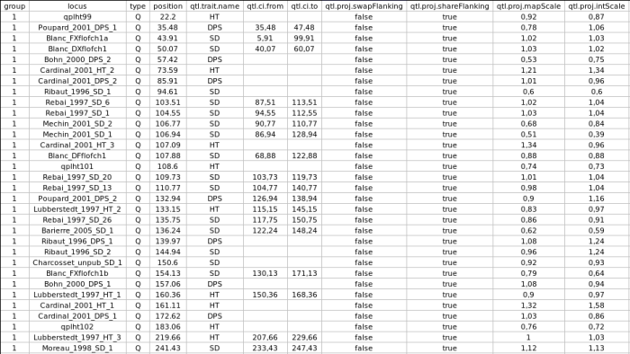
The attributes qtl.ci.from and qtl.ci.to gives the new confidence interval of the QTL when a confidence interval exists in the intial mapping experiment. This new confidence interval is computed according to the projection scale given by the homothetic ratio gvien by the attribute qtl.proj.mapScale, while the position of the QTL is computed relatively to the flanking markers using the homothetic ratio given by the attribute qtl.proj.intScale. The boolean attributes qtl.proj.shareFlanking and qtl.proj.swapFlanking indicate for the former that the QTL flanking markers are observed into both the intial and the consensus map, and the later will be true if these markers are observed in a reverse order between the two maps.

Note that for half of the QTL in chromosome 1 there is no information about the CI. Nevertheless, if you look at the file consensus_qtl.txt you will see another field called qtl.rsquare which gives the percentage of variance explained by the QTL (this field was not included in the above table) and from which a theoretical confidence interval could be computed according to the mapping population properties (size and type of cross: these two parameters are given by the attributes qtl.cross.size and qtl.cross.type).